AirBnB Price Estimation with Machine Learning

Using regression machine learning to estimate and suggest a price of AirBnB listings


Abstract

AirBnB offers a service to their hosts in which they suggest an ideal price for a listing. The purpose of this service is to help AirBnB hosts choose a price that will result in the most success for that listing. AirBnB made their New York City data available publicly to challenge developers in making such an algorithm in the hopes that some developers can find ways to improve this process. In this project, I explore various concepts in AI and data analytics to attempt to better predict and estimate prices of listings.

Data

The data of this project is provided by AirBnB and can be found in the repository. The data contains approximately 50,000 listings from New York City; the format of this structured data can be seen on the right. While the data is comprehensive and provides adequate information about each listing, certain information is missing from some of the samples. As such, data cleaning was a necessary first step; the manner in which this cleaning is done and the code to do it are outlined in the data processing notebook.
id name host_id host_name neighbourhood_group neighbourhood latitude longitude room_type price minimum_nights number_of_reviews last_review reviews_per_month calculated_host_listings_count availability_365
0 2539 Clean & quiet apt home by the park 2787 John Brooklyn Kensington 40.64749 -73.97237 Private room 149 1 9 2018-10-19 0.21 6 365
1 2595 Skylit Midtown Castle 2845 Jennifer Manhattan Midtown 40.75362 -73.98377 Entire home/apt 225 1 45 2019-05-21 0.38 2 355
2 3647 THE VILLAGE OF HARLEM....NEW YORK ! 4632 Elisabeth Manhattan Harlem 40.80902 -73.94190 Private room 150 3 0 NaN NaN 1 365
3 3831 Cozy Entire Floor of Brownstone 4869 LisaRoxanne Brooklyn Clinton Hill 40.68514 -73.95976 Entire home/apt 89 1 270 2019-07-05 4.64 1 194
4 5022 Entire Apt: Spacious Studio/Loft by central park 7192 Laura Manhattan East Harlem 40.79851 -73.94399 Entire home/apt 80 10 9 2018-11-19 0.10 1 0

Data Visualization

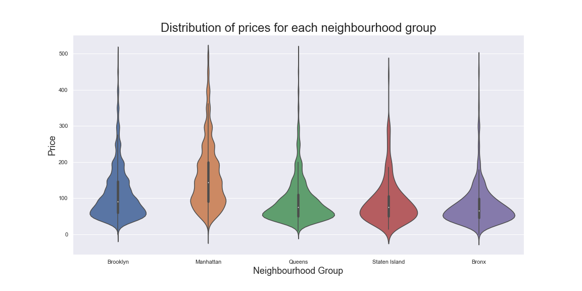
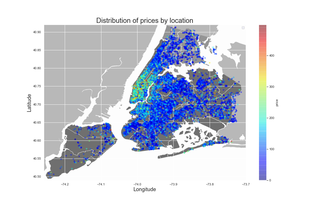
We can visualize the data in various ways to attempt to understand it. Below, we visualize the price distribution in each borough or neighbourhood group to see the relationship between prices and borough. This figure shows that while all boroughs have expensive properties, some, like Queens and Bronx, have a larger portions of cheaper properties. Contrarily, Manhattan seems to have higher portions of more expensive properties. This figure also shows that the neighbourhood group is an important feature for the model that can help it estimate an ideal price for the listing. Another important feature is the specific location or coordinates of the listing. As shown by the first figure on the right, the location of the listing impacts it's price; as such, certain areas have a higher concentration of expensive listings.
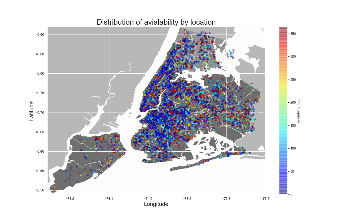
Another attribute that can be visualized is the availability accross the map. This is shown in the second figure on the right.
Feature Analysis

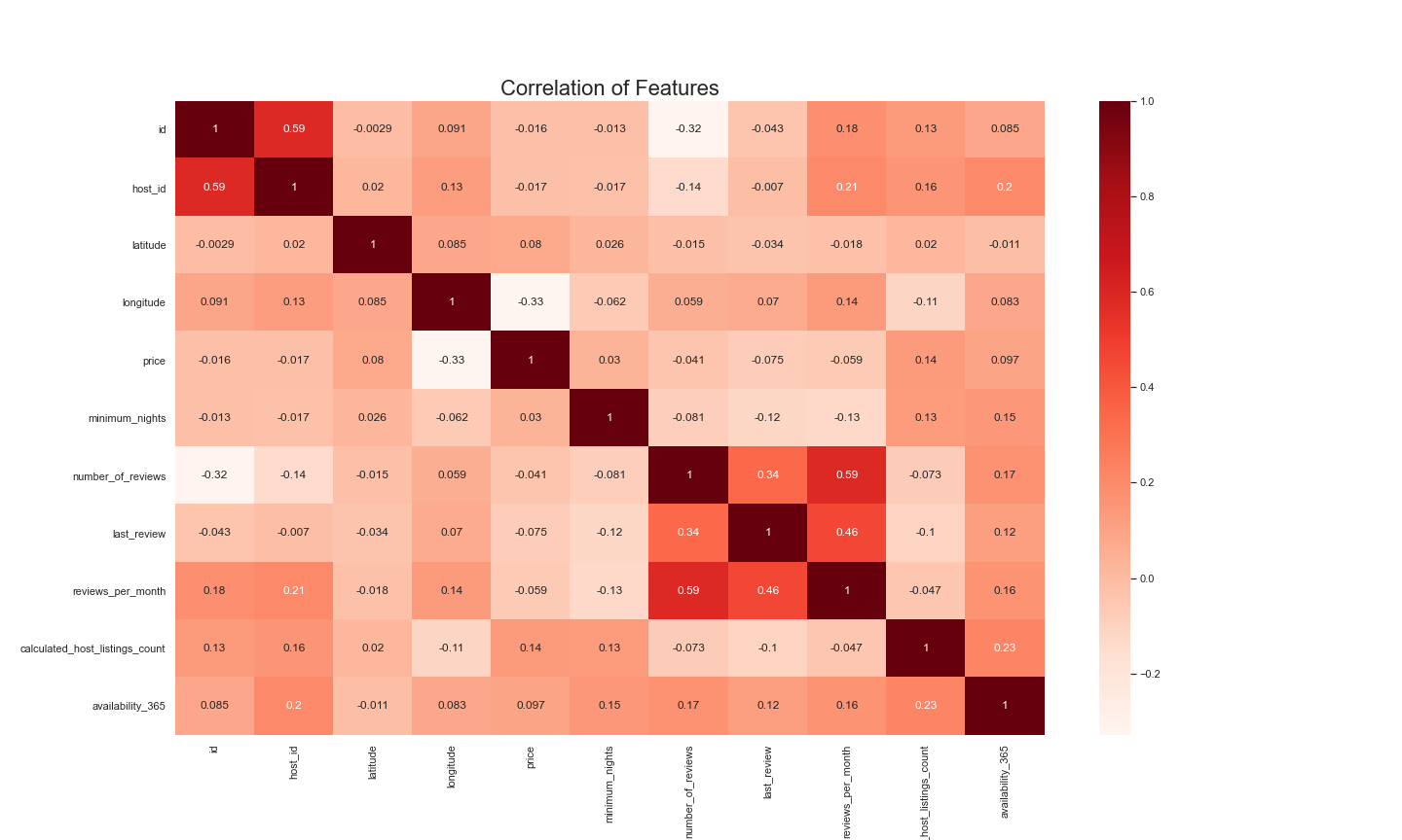
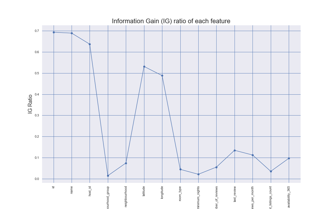
We continue to analyze the data by looking at the correlation of features by looking at pearson correlation, shown in the heatmap in the figure below on the left, and the information gain (IG) ratio shown in the figure on the right. The correlation heatmap indicates how closely related each two features are. With the exception of the identification features, "id" and "host_id", all the features seems to be independent of each other. The IG ratios in the figure on the right show the importance of each figure in terms of its correlation to the listing price. Once again, we see the identification features have the highest weight. Other important features are the coordinates.

Feature Engineering and Data Cleaning

Feature engineering is critical for obtaining good results from ML models; unprocessed data can be extremely difficult for algorithms to learn. The most important part of feature engineering in this application is the price distribution. As can be seen in data visualization above, the price distribution tends to be very uneven with some very high-priced listings that can be outliers in the data. Such outliers will make it more challenging for algorithms to find patterns in the data. Therefore, applying a logairthmic transformation, as seen in the figure below, helps make the distribution appear closer to a normal or Gaussian distribution, which is typically easier for algorithms to learn. Other forms of feature engineering done in this project include changing features like neighbourhood group into categorical features and adding an extra feature for availability highlighting the importance of yearly-round available listings.
Data cleaning can also help improve performance. Data cleaning includes removing certain features like id and host name as well as removing certain samples that do not have enough information and might mislead the model. Samples that continue to lie outside the price distribution curve, after the logarithmic transformation, were also removed to help the model better recognize the overall pattern. The full procedure of feature engineering and data cleaning, along with the code, can be found in the data processing notebook.

Machine Learning Model

Basic Regressors

We begin by testing the most common basic regression models. Six models are tested with default parameters as an initial test. The test utilizes 5-fold cross-validation to ensure consistency in the performance. The table to the right shows the results of this test in which the performance is measured using Mean Squared Error (MSE). Results show that the top three performers are Ridge, Lasso, and Random Forest regressors.
Model Mean MSE Standard Deviation
Linear Regression 23.034 x 10¹² 34.6613 x 10¹²
Ridge Regression 0.20207 0.002854
Lasso Regression 0.45251 0.005495
Elastic Net 0.45181 0.005455
Random Forest Regression 0.18457 0.004537
Huber Regression 0.21558 0.006004

Parameter Optimization

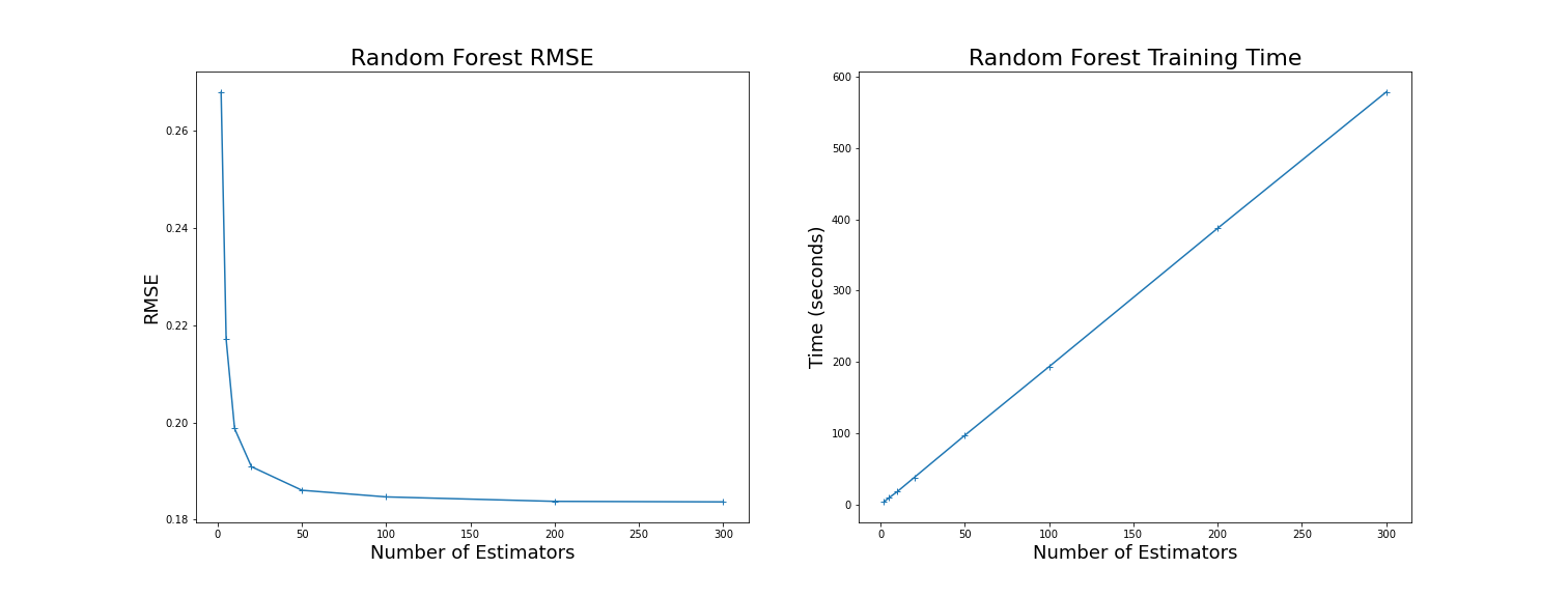
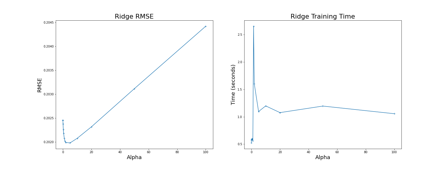
We test the top three models from the previous section with varying parameters. We perform this test by re-training each model with varying parameters and measuring the corresponding MSE of the test data. The two figures below shot plots of MSE and training time with varying the main parameter. The main parameter of the Random Forest regressor is the number of estimators, and the main parameter of Ridge regressor is alpha which is a factor that reduces the variance of the estimates from the model.
Huber Regressor was also tested for varying parameters. These parameters are alpha, the regularization parameter and epsilon which controls the number of samples that should be classifierd as outliers. The most optimal parameters and the corresponding results are outlined in the table below.
Model Parameters MSE
Ridge Alpha = 5 0.195635
Random Forest Number of estimators = 50 0.177121
Huber Alpha = 10, Epsilon = 3 0.207392

Ensemble Learning

We utilize ensemble learning to combine the strengths of multiple models. This concept is based on the idea that some regressors are better at modelling certain data types than others. As such, multiple regressors are trained on the same data and the output of all the models is averaged to produce the final output. In this case, we can combine the three models from above to make an ensemble model. The result is superior performance than the individual models alone.
Model MSE
Ensemble Model 0.173568
The detailed process of constructing these models and the code can be found in the github repository

Final Remarks

The results of this experiment show the promising capabilities of estimating prices of house listings using machine learning models. A key takeaway from this project was the importance of data processing and feature engineering. As an example, testing the Random Forest regressor used in this experiment without feature engineering produced far worse results as can be seen in the table below.
Without Feature Engineering With Feature Engineering
38934.3 0.177121